Relatively simple models can be built from just a handful of parameters. The parameters get updated as better information comes in, and the model updates with them. I want to walk through where the core equations come from, define the number everyone kept quoting during COVID (\(R_0\)), and then actually simulate the thing in Python so the curves aren’t just abstract.

A short history

Early disease modeling traces back to physicists, of all people. Daniel Bernoulli, better known for fluid dynamics, derived an early epidemiological model describing smallpox spread through a population, back when variolation (an early, crude form of smallpox vaccination) was showing some real efficacy at controlling outbreaks.

Modern infectious disease modeling has its core in the SIR model, a compartmental model: Susceptible, Infectious, Recovered/Removed. In its most basic form, with only those three categories, it shows how an infectious agent propagates through a population as a function of time.

Setting up the model

Take a population of size \(N\), and split it into three groups: \(S\), \(I\), and \(R\). To make the math easier, assume the population size stays constant (an oversimplification, but a fine starting point). Each group is a proportion of the total, and each group is a function of time:

Since each term here is a proportion, we can drop the \(N\) and write the lower case versions instead: \(s(t)\), \(i(t)\), \(r(t)\). What we actually care about is how these functions change over time, so we differentiate each one to get the instantaneous rate of change, moving from discrete to continuous time along the way.

There has to be some transfer of people from the susceptible group into the infectious group. That transfer rate is governed by \(\beta\), the probability that a susceptible person becomes infected on contact with an infectious one. There also has to be a transfer from infectious to recovered, governed by \(\gamma\), which is inversely proportional to how long a person stays infectious. In this simple version of the model, a person stops being infectious whether they recover or die; the model doesn’t distinguish between the two. (More realistic versions handle re-entry into the susceptible pool after recovery, or after a period of immunity wears off, but that’s an extension for another post.)

Putting the parameters together with the groups gives the classic system of nonlinear ordinary differential equations:

Solving this system gives the epidemic curve, once \(\beta\) and \(\gamma\) are pinned down. The catch is that these constants aren’t universal. They shift depending on the pathogen, the season, and how the population is behaving, so any solution is only as good as the parameter estimates feeding it.

The number everyone kept citing: R0

One term worth defining on its own is the basic reproductive number, \(R_0\): the average number of people each infected person goes on to infect. If \(R_0 > 1\), the disease is in an epidemic state and growing exponentially. If \(R_0 = 1\), it’s endemic, holding roughly steady in the population. If \(R_0 < 1\), it eventually dies out on its own.

Estimates for SARS-CoV-2’s \(R_0\) landed somewhere between 2 and 3.5, which is a wide enough range that it produces a wide range of outcomes once you plug it into a compartmental model. It’s also worth noting that \(R_0\) isn’t a fixed property of the virus. It shifts with behavior (mask-wearing, distancing) and with therapeutics: a shorter illness duration lowers it, all else equal. This leads to a genuinely counterintuitive result: a disease that killed within a day or two would, mechanically, have a lower \(R_0\) than one that let people walk around infectious for two weeks, simply because there’s less time to spread it.

Simulating it

None of this needs anything exotic. scipy.integrate.odeint will solve the system directly given the three equations above, starting conditions, and a time range.

import numpy as np
from scipy.integrate import odeint
import matplotlib.pyplot as plt

def sir_model(y, t, beta, gamma):
    s, i, r = y
    ds_dt = -beta * s * i
    di_dt = beta * s * i - gamma * i
    dr_dt = gamma * i
    return [ds_dt, di_dt, dr_dt]

# Parameters
r0 = 2.0
gamma = 1 / 10  # infectious for about 10 days on average
beta = r0 * gamma

# Initial conditions: proportions of the population
i0 = 1e-5
s0 = 1 - i0
r0_init = 0
y0 = [s0, i0, r0_init]

t = np.linspace(0, 250, 500)

result = odeint(sir_model, y0, t, args=(beta, gamma))
s, i, r = result.T

peak_day = t[np.argmax(i)]
peak_fraction = np.max(i)

print(f"R0: {r0}")
print(f"Peak infected fraction: {peak_fraction:.4f}")
print(f"Peak occurs at day: {peak_day:.1f}")

plt.figure(figsize=(8, 5))
plt.plot(t, s, label="Susceptible")
plt.plot(t, i, label="Infectious")
plt.plot(t, r, label="Recovered")
plt.xlabel("Days")
plt.ylabel("Fraction of population")
plt.title(f"SIR model, R0 = {r0}")
plt.legend()
plt.tight_layout()
plt.savefig("sir_simulation.png", dpi=150)

Running this with \(R_0 = 2\) produces the familiar shape: susceptible drops off, infectious spikes and then decays, recovered climbs and plateaus. Because the whole population was never infected before the disease burned itself out, susceptible doesn’t bottom out at zero; there’s a chunk of people who never got exposed at all.

Bump \(R_0\) up toward 3.5 and rerun it, and the peak gets both taller and earlier. That’s the entire mechanism behind flattening the curve: lowering \(\beta\) (through distancing, masks, closures) lowers the effective \(R_0\), which pushes the peak lower and later, giving healthcare systems more room to keep up.

Where the simple model breaks down

The basic SIR model assumes uniform mixing: every susceptible person is equally likely to bump into every infectious person, which isn’t how real populations behave. People cluster around shared destinations (a workplace, a campus, a grocery store), and that clustering matters a lot for how fast a disease actually spreads, even when the aggregate contact rate looks the same on paper.

A more realistic model needs to account for that structure, plus a few other things this version leaves out entirely: travel between otherwise separate communities, reinfection after immunity wears off, and different transmission probabilities for asymptomatic versus symptomatic carriers. 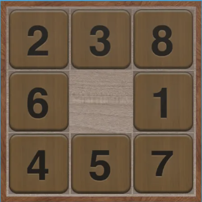Each of those turns three coupled equations into something considerably messier, but the same core idea holds: get the parameters right, and the model tells you, quantitatively, what a given policy or behavior change is actually going to do to the curve.

Slide tiles into the blank space until the numbers run 1 through 8 in order, with the blank in the top left.

Does the textbook hierarchy of state space search algorithms actually behave the way the textbooks claim on a problem small enough to inspect by hand? That’s what I wanted to find out here. The Eight Puzzle is the canonical toy. A 3x3 grid with eight numbered tiles and a single blank, and the goal is to slide tiles into ascending order with the blank in the top left. The reachable state space has size 181,440, which is exactly half of 9! because tile slides preserve permutation parity.

So do random, breadth first, depth first, greedy best first, and A* search separate cleanly on this problem, and how much of the separation comes from the algorithm versus the heuristic you give it?

The problem is that the state space, while finite, is large enough that uninformed search wastes most of its work on configurations no human solver would ever consider. A blind frontier expansion at depth 18 still has roughly \(3^{18}\) candidates if you ignore cycle detection, which is around 387 million.

Even after pruning cycles the count stays in the millions on the harder boards. Any algorithm that does not somehow weight the search toward goal-like states is going to spend almost all of its budget visiting irrelevant ones. That is the case for heuristic search. The flip side is that a poorly chosen heuristic can make things worse than no heuristic at all, by confidently steering the search down a corridor that does not lead to the goal.

It’s a bit hard to explain the exact code implementation, so contact me if you want a more detailed explanation and I’d be happy to talk about it. The gist is this:

The dataset is three text files of starting configurations, grouped by the optimal solution length: 5_moves.txt, 18_moves.txt, and 27_moves.txt. Each file has ten boards encoded as a permutation of the digits 0 through 8, where 0 is the blank. The optimal length is the labeled difficulty. The 5 move set is for sanity checks. The 18 move set is the regime where uninformed search is on the edge of feasible. The 27 move set is past it.

The first thing you have to decide is how to represent a board. I went with a 2D list of integers and tracked the blank position explicitly as (blank_r, blank_c) so I never have to scan for it.

The constructor takes a 9 character digit string and fills the grid row by row.

Tracking the blank position is not strictly necessary but it converts every move from \(O(n)\) to \(O(1)\), and over millions of generated successors that is a huge benefit.

A move slides the blank in one of four directions. Internally I shift the blank coordinate, check it stays inside the grid, and if so swap the blank with the tile that was there:

where \(d \in {(-1, 0), (1, 0), (0, -1), (0, 1)}\) for up, down, left, right. If the new coordinates are off the grid, the move is rejected.

A State wraps a Board with three extra fields: a predecessor pointer, the move that produced this state, and the depth in the search tree.

The predecessor pointer is what lets me reconstruct the move sequence at the end without storing the full path inside the state. It also lets me detect cycles incredibly easily by walking back up the chain and checking for board equality.

This matters because without cycle detection, even BFS will waste time re-expanding the same configurations.

Successor generation tries all four directions on a copy of the board, keeps the moves that succeed, and wraps each into a new State with the predecessor set to self.

The branching factor is at most four, typically two or three after cycle pruning.

The search abstraction is a Searcher base class with a list of untested states, a depth limit, and a tested counter. The contract is that find_solution pops a state via next_state, checks goal, generates successors otherwise, and adds them subject to a should_add filter that enforces the depth limit and rejects cycle creators.

Subclasses override next_state to implement different orderings: random pick for the base class, FIFO for BFS, LIFO for DFS, and a priority-max pick for the informed searchers.

There is a real argument for just running BFS and calling it done, because BFS is complete and optimal for unit-cost step problems, and the Eight Puzzle is one.

The question is whether you can do better in states tested without giving up optimality. That is what informed search is supposed to deliver. An admissible heuristic should let A* prune the frontier without ever closing off the optimal path.

The heuristics I implemented are non standard and worth describing. h0 returns 0, which makes A* behave like uniform cost search. h1 returns state.num_moves, which is the g cost and not a heuristic in the usual sense. h2 returns num_moves plus the Manhattan distance of the blank from the origin (0, 0).

Neither h1 nor h2 estimates the distance from the current state to the goal in the way a textbook heuristic would. I left them in because the experiments they enable still illustrate the point: any monotone signal that grows with depth or distance from a fixed reference biases the search, and the bias either helps or hurts depending on whether the signal correlates with proximity to the goal.

One thing to be upfront about: h1 and h2 are not admissible. Both include g, the number of moves already made, and that can easily be larger than the number of moves left to the goal. So the textbook optimality guarantee for A* does not formally apply to them. As you’ll see below, A* with h2 still returns optimal solutions here, but for a different reason.

The Greedy searcher computes priority as

with h treated as zero unless the heuristic is h2, in which case it is added.

The negation is there because I take max over priorities to pick the next state. Misplaced tile count, defined as the number of tiles not in their goal position, ends up doing basically everything Greedy. It is a real heuristic in the textbook sense, and Greedy with misplaced tile count finds solutions quickly but rarely optimally.

The A* searcher computes priority as

which is the negated f-cost from the textbook formula \(f = g + h\), if you read num_moves as g and h as the heuristic.

The catch is that with h1 the h term is itself num_moves, so f effectively doubles g and the search degenerates into BFS with a strange tiebreaker.

With h2 things improve, because the blank distance term breaks ties in a way that prefers states whose blank is closer to the top left corner, which is where the goal puts it. On these particular puzzles that correlates with progress.

Notice that 2g goes up by 2 with every move, while the blank term only ranges from 0 to 4. So A* with h2 still mostly expands states in order of depth, like BFS, with the blank position deciding the order within and between neighboring depths. That is why it keeps finding optimal solutions even though h2 isn’t admissible.

Now to the results:

On 5_moves.txt every algorithm solves every puzzle. The interesting numbers are states tested. BFS expands on the order of a hundred to a few hundred states per puzzle. DFS with no depth limit can dive deep and tested counts are either small or huge depending on the seed. Greedy with misplaced tiles finishes in tens of states. A* with h2 finishes in similar territory. At this difficulty the algorithms are indistinguishable from a solving perspective.

On 18_moves.txt the separation between algorithms appears. BFS finishes but the expanded frontier crosses 100,000 states on the harder boards. DFS with a depth limit of 20 sometimes returns a 20 move solution and sometimes runs out of frontier without finding one. Greedy with the misplaced tile count finds solutions quickly but they are bad: 92, 56, 66, 186, 194, 96 moves on the puzzles it solves, against an optimal of 18.

That is what greedy looks like. It commits to the first frontier expansion that scores well and then meanders.

A* with h2 gives the best results of the bunch. On the six boards it solves within a reasonable interrupt threshold, every solution is exactly 18 moves, and the states tested counts are 34413, 32283, 46097, 32009, 39396, 33053.

Compare to the BFS frontier on the same problem and A* tests fewer states on average. More importantly, every solution it returns is optimal, which Greedy never guarantees.

The four boards it does not solve are ones where I ran out of patience and interrupted the search rather than ones where the algorithm failed in principle.

Algorithm comparison across difficulty levels. BFS and A track each other on optimality. Greedy diverges as soon as the optimal length crosses the easy threshold.*

The 27_moves.txt file is past the point where any of these algorithms reach a solution in a reasonable wall clock time without a much stronger heuristic. A heuristic that does not estimate distance to goal cannot, in general, prune deep enough to reach a 27 move target. If I wanted to push the difficulty further I would replace h2 with the sum of Manhattan distances of every tile from its goal position, which is admissible and well known to be effective on this problem.

It is worth asking whether the algorithm comparison generalizes. The answer is mostly yes. BFS is optimal but computationally expensive. DFS is computationally cheap but unreliable without an extremely good depth limit. Greedy is fast but lossy on solution quality. A* with an admissible heuristic is the one that guarantees optimality while searching less than BFS, and it pays for that with sensitivity to the heuristic.

The “searching less” part needs a caveat. If the heuristic is also consistent (it never drops by more than 1 across a single move), A* never expands more states than uniform cost search, ties aside. That isn’t a guarantee for every heuristic, and it’s not what my h2 runs show, since h2 is neither admissible nor consistent. The smaller counts I got come from the tiebreaking described above.

The 8-puzzle is small enough that you can see all four behaviors on a single laptop in a few minutes of runtime.

The A* with h2 numbers on 18_moves.txt make informed search look like an obvious win, but they don’t tell the whole story. On the boards it failed to solve in the same file, the blank’s position happens to be a poor proxy for true distance to the goal. On those, the priority queue keeps preferring states that score well by the heuristic but are actually further from the goal in moves.

Replacing the heuristic with sum of Manhattan distances might close the gap. It might be something I look into as an extension to this in the future.

The natural extensions from here are obvious. Implement the standard admissible heuristics inside A* (misplaced tiles without the g term, total Manhattan distance, linear conflict). Add iterative deepening A*, which trades memory for some redundant work and can solve 27 move boards on a laptop. Move from the 8-puzzle to the 15-puzzle, where the state space jumps from 181K to roughly \(10^{13}\) and uninformed search is no longer an option at all.

The result of this exercise is that the algorithm hierarchy mostly behaves as expected, and that the heuristic matters as much as the algorithm. Even a weak heuristic like h2 was enough to beat BFS in the 18 move regime, but not enough to push to 27. That needs a heuristic that actually estimates distance to the goal.

We are enjoying a planetary parade during the beginning of this month here on Earth, but my alien friend from the distant planet Pyrknot (well modeled as a perfect sphere) isn’t too impressed. Their single-star system has six planets other than Pyrknot with such chaotic orbits that each night these planets independently appear in uniformly random locations in the Pyrknothian sky (the planets aren’t visible in daylight). If at a given moment there exists somewhere on Pyrknot that all six planets are visible, then from my friend’s position on the surface they have an \(\alpha\) probability of also seeing all of the planets.

My friend is considering building a tower to improve their chances of seeing these planetary parades. Assume the tower allows the viewing of every celestial body that could be seen from at least one location on the surface of Pyrknot less than a distance \(r\) from the base of the tower. In the limit of \(r\) being small compared to the radius \(R\) of Pyrknot, the new probability of seeing the planetary parade from the top of the tower is linearly approximated by \(\alpha + \beta \cdot (r/R)\). Find \(\alpha\) and \(\beta\) in exact terms.

Ok, so now we know the problem. I want to work through computing the probability that my friend on Pyrknot sees a planetary parade, both from the surface and from the top of a small tower. The setup is that Pyrknot is a perfect sphere with radius \(R\), orbiting a single star, and sharing its system with six other planets. Each night those six planets appear independently at uniformly random locations in the sky, and none of them are visible in daylight. The question asks for the probability \(\alpha\) that my friend can see all six planets given that someone on the surface can, and then there’s the linear correction \(\beta \cdot (r/R)\) that a tower of effective radius \(r\) provides.

The first thing you need to figure out is the geometry of who can see what. From any point on the surface of a perfect sphere, you can see exactly one hemisphere of the sky. That means every celestial body (don’t forget the seventh body: the star!) defines a great circle on the surface of alien planet. On one side of that great circle, the body is above the horizon. On the other side it’s the opposite. So the problem of figuring out which surface points can see which bodies reduces to understanding how seven great circles partition the sphere.

This already seems extremely difficult, but actually the partitioning is pretty easy if you happen to know Euler’s formula for a sphere, \(V - E + F = 2\). Every pair of great circles intersects at exactly two antipodal points, so the vertex count is

\[V = 2 \binom{7}{2} = 2 \times 21 = 42\]

Each of the seven great circles gets cut into arcs by its intersections with the other six. That is \(6 \times 2 = 12\) intersection points per circle, which means 12 arcs per circle, giving

\[E = 7 \times 12 = 84\]

and therefore

\[F = 2 - V + E = 2 - 42 + 84 = 44\]

There are 44 regions on the surface of Pyrknot, each of which sees a subset of the seven bodies. For a planetary parade to be visible from a region, that region needs all six planets above the horizon and the star below the horizon. At most one region can satisfy this at any given moment. By symmetry all 44 regions have the same expected area, so conditional on a parade existing somewhere, my friend is in the correct region with probability \(1/44\). That gives \(\alpha = 1/44\).

Now for the tower, and it’s worth noting that there is some trickiness that comes in because of that daylight blocking out the planets stipulation that was stated in the question.

The tower lets my friend see any celestial body that is visible from at least one surface point within distance \(r\) of the base. To first order in \(r/R\), this is equivalent to pushing the boundary of their region outward by \(r\) in every direction. The region gains a strip of area along its perimeter, and the area of that strip is approximately the perimeter times \(r\).

The next question is what the expected perimeter of a single region is. The 7 great circles have a combined length of \(7 \times 2\pi R = 14\pi R\). Every arc segment borders two adjacent regions, one on each side, so when you add up the perimeters of all 44 regions, each arc gets counted twice:

\[\text{total perimeter} = 2 \times 7 \times 2\pi R = 28\pi R\]

By symmetry, the expected perimeter of a single region is

\[\bar{P} = \frac{28\pi R}{44} = \frac{7}{11}\pi R\]

This is where some details actually change the answer. Not every boundary segment helps. Of the seven great circles, six come from planets and one comes from the star. When the tower pushes past a planet boundary, it lets my friend see an additional planet they could not see before. That is good, but when it pushes past the star boundary, it means the top of the tower is now in daylight, and the parade is ruined. So the star boundary actually shrinks the region we’re interested in instead of expanding it.

By symmetry, \(6/7\) of the expected perimeter comes from planet boundaries and \(1/7\) comes from the star boundary. The net first order change in area is

\[\Delta A = \frac{6}{7} \cdot \frac{7}{11}\pi R \cdot r - \frac{1}{7} \cdot \frac{7}{11}\pi R \cdot r = \frac{6}{11}\pi R r - \frac{1}{11}\pi R r = \frac{5}{11}\pi R r\]

As a fraction of the total surface area \(4\pi R^2\):

\[\frac{\Delta A}{4\pi R^2} = \frac{(5/11)\pi R r}{4\pi R^2} = \frac{5}{44} \cdot \frac{r}{R}\]

So the linearized probability of seeing the parade from the tower is

\[P = \frac{1}{44} + \frac{5}{44} \cdot \frac{r}{R}\]

which gives \(\alpha = 1/44\) and \(\beta = 5/44\).

There is more to say about what happens when \(r\) is not small relative to \(R\), and whether the linear approximation remains useful at larger tower sizes.

The problem is that CPI is an aggregate of thousands of individual prices across categories that move for completely different reasons: energy prices respond to geopolitics and OPEC supply decisions, shelter costs follow the housing cycle with a long lag built into how the BLS measures rent, food prices track agricultural commodities and supply chains, and a long list of other variables to consider. Any model that tries to forecast the aggregate has to somehow learn these dynamics from a single target series, which is part of why naive autoregressions are hard to beat.

The dataset is FRED MD, the monthly database maintained by the St. Louis Fed. It has something like 120 macro and financial series including industrial production, employment by sector, exchange rates, treasury yields at various maturities, money supply aggregates, commodity prices, and a long list of other things. After loading the file there are 690 monthly observations.

The first thing you have to figure out is that almost none of these series are stationary. CPI has trended upward for seventy years. Industrial production grows, the money supply grows. If you feed the level of a trended series into any model, the model will spend most of its capacity learning the trend instead of the relationships you actually care about. So before doing anything else I first difference every feature column:

and I define the supervised target as the h step change in the level of CPI:

For the experiments here \(h = 1\), but the code is parameterized for any positive horizon. The choice to predict a difference rather than a level is one I will return to when I get to the results, because it ends up mattering much more than it might look at first.

The next and first genuinely interesting problem to consider is that with around 120 candidate features and only 689 rows of usable data, you will absolutely overfit if you hand the network everything at once. So I run a three stage feature selector, fit only on the training portion of the data:

Another way of explaining this: drop near constants, then keep the top \(K_1 = 60\) features by absolute Pearson correlation with the target delta, then refine to the top \(K_2 = 30\) features by Random Forest importance. The reason for the cascade rather than a single criterion is that correlation is a cheap linear filter while a Random Forest captures nonlinear and interaction effects but is computationally expensive to fit on a wide matrix. Doing the cheap filter first makes the more expensive RF stage tractable. An important detail is that the selector is fit only on rows whose target time also falls inside the training window. If you fit it on the full sample, you have already leaked information about future inflation into the feature set, and every metric you report afterward is not useful (it’s nonsense).

It is worth asking whether the features the model selected make any economic sense. Among the top 30 by Random Forest importance, I would expect to find variables related to energy prices, labor market indicators, interest rate spreads, and money supply growth. If the selector is instead picking up series with no plausible link to inflation, then it might be a signal the model is fitting noise. I did not tune the selector to enforce selecting certain features, so whatever it picks is a revealed preference of the data. But the interpretation cuts both ways: a model that selects economically sensible features and still cannot beat a naive baseline is telling you that the signal to noise ratio in monthly macro data is genuinely low, and no amount of architecture will fix that.

The next question is what model to use. There is a real argument for just running an autoregression on the differenced CPI series, because it seems that inflation has strong autocorrelation and most of the predictable variance in next month’s CPI is in last month’s CPI. But macro series interact with each other in ways that are not necessarily contemporaneous. A change in oil prices today may not show up in headline inflation for several months, and the size of the effect depends on the state of demand and inventories. An LSTM can in principle learn these lagged, state dependent relationships from the sequence directly, without me having to specify a fixed lag structure ahead of time. That is the bet I’m making.

The network itself is a two layer LSTM with hidden size 64 and dropout 0.20, followed by a small feed forward head. Some basic LSTM architecture as a refresher below: At each time step the LSTM cell computes the standard set of gates:

where \(f_t\), \(i_t\), \(o_t\) are the forget, input, and output gates, \(\tilde{c}_t\) is the candidate cell update, \(c_t\) is the cell state, \(h_t\) is the hidden state, and \(\odot\) is elementwise multiplication. After running the input window of 24 months through the LSTM, I take the final hidden state \(h_T\) and pass it through a two layer head:

where \(W_1 \in \mathbb{R}^{32 \times 64}\) and \(W_2 \in \mathbb{R}^{1 \times 32}\). The output \(\hat{y}\) is the predicted standardized delta. To recover the level prediction at time \(t + h\), I undo the standardization and add the known anchor:

This anchoring step is the entire reason the level metrics look so good. I’ll have some more info on that later.

Training uses Adam with learning rate \(10^{-3}\), weight decay \(10^{-5}\), gradient clipping at norm 1.0, and early stopping on validation MSE with a patience of 15 epochs. The loss is mean squared error on the standardized delta:

The split is chronological: the first 70% of observations are training, the next 15% are validation, the final 15% are test. This is non negotiable for time series. Random shuffling here would let the model see futures it should not have access to, which is a different flavor of the same leakage problem the feature selector has to avoid.

When you train this, the validation loss bottoms out around epoch 13 and then drifts upward, and the early stopping kicks in around epoch 28. Train MSE keeps falling all the way down to roughly 0.14 in standardized units while validation MSE sits around 7.3 at its best. That gap is large and it is a signal that the model is memorizing the training period more than it is learning generalizable structure. And to be blunt about what 7.3 means: the target is standardized, so a model that always predicts the training mean would score an MSE of about 1. On the validation period, the LSTM is doing worse than that.

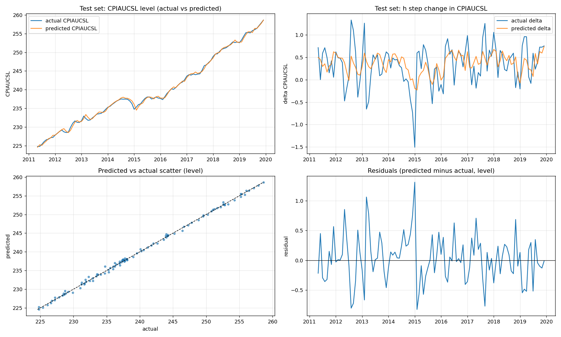
Now to the results, and the part that people should probably be wary of. When I plot the predicted CPI level against the actual CPI level on the test set, the two lines mirror each other almost perfectly. Level RMSE on the test set is 0.39 and level MAPE is 0.125%. If you stopped reading at that plot you would conclude the model is excellent.

Test set predictions and residuals. The level plot in the top left looks great. The delta plot in the top right is the one to actually look at.

The level plot flatters the model. The two lines hug each other because most of \(\text{level}[t+h]\) is just \(\text{level}[t]\), which the model is handed for free: it only has to predict the change and add it to this month’s known CPI value.

The plot that actually tells you something is the delta plot, the predicted h step change against the actual h step change. This is where the model has to earn its keep, and the delta MAPE is 140% because actual deltas are often very close to zero and ratios blow up. The delta RMSE is 0.39, which is the same number as the level RMSE, and that is the point. The level RMSE is just the delta error sitting on top of a perfectly known value. Decompose like this:

The level error is identically the delta error. Reporting the level metric without the delta metric is basically a magic trick.

This is also where the black box question comes in. An LSTM with 60,000 parameters is not interpretable in the way a regression coefficient is interpretable. You cannot point at a number and say “a one standard deviation increase in industrial production raises forecasted inflation by such and so.” You can run permutation importance on the inputs after training, you can compute integrated gradients along the input sequence, you can run partial dependence on a single feature while holding the others at their median. All of those are post hoc and approximate.

The natural next question is whether this approach extends to longer horizons, and whether you can get cleaner generalization by changing the inductive bias.

There are also obvious modifications to the architecture: attention over the input window, a state space layer in place of the LSTM, a probabilistic head that returns a distribution rather than a point estimate. Each of these changes the bias variance tradeoff in a different direction.

So where does this leave the original question? Honestly, this version doesn’t answer it yet. The level metrics look great for reasons that have nothing to do with the LSTM, the validation loss is worse than predicting the mean, and I haven’t put a simple autoregression on the same test set to compare against. That comparison is the next thing to do: fit an AR(p) and a random walk (predict a change of zero) on the differenced CPI series and report their delta RMSE next to the LSTM’s. Until the LSTM beats those, the honest conclusion is that monthly macro data is noisy enough that the extra machinery isn’t paying for itself. I still think there’s room for neural networks here, probably alongside econometric methods rather than instead of them, but this post is a starting point and not proof.

Before getting into the details, I want to note that some of the context required to fully appreciate what is going on here, particularly around how the contracts are selected and how the ARIMA step works, will have to come in later posts. That said, I am going to try to give as much useful detail as I can here so that the overall picture is at least clear. And it goes without saying that some important details I can’t share due to the proprietary nature of the work involved.

The naive approach is to fit a time series model directly to the IV of each contract and forecast forward. The problem is that IV series are noisy, non-stationary in complicated ways, and each contract has its own dynamics depending on its strike, tenor, and the underlying’s behavior at that point in time. A single model fit across everything tends to perform poorly.

The approach I took instead is a hybrid: use ARIMA to capture the smooth, mean-reverting component of each contract’s IV trajectory, and then train a separate XGBoost model to predict the residuals that ARIMA gets wrong. The final forecast is just the sum of the two.

The idea is that ARIMA handles the trend and autocorrelation structure reasonably well, but it has no way to incorporate cross-sectional information like IV skew, tenor, or the day of the week. XGBoost can learn those patterns from the residuals across all contracts simultaneously.

The ARIMA(p, d, q) model expresses the differenced series as a linear combination of its own past values and past forecast errors:

\[\Delta^d y_t = c + \sum_{i=1}^{p} \phi_i \Delta^d y_{t-i} + \sum_{j=1}^{q} \theta_j \varepsilon_{t-j} + \varepsilon_t\]

where \(\phi_i\) are the autoregressive coefficients, \(\theta_j\) are the moving average coefficients, \(d\) is the order of differencing, and \(\varepsilon_t\) is white noise. The orders \(p\), \(d\), and \(q\) are selected separately per contract by minimizing an information criterion.

The pipeline works as follows. For each options contract, I split the observed IV history into a fit window and a validation window. ARIMA is fit on the fit window, and its out-of-sample forecasts over the validation window give both a predicted trajectory and confidence intervals. The difference between those forecasts and the actual observed IV is the residual:

\[r_t = y_t - \hat{y}_{\text{ARIMA}, t}\]

and that residual becomes the target for XGBoost.

The features I pass to XGBoost are things that are available at inference time. The lagged residuals are important because ARIMA residuals tend to be autocorrelated in ways that ARIMA itself does not fully capture, and XGBoost can exploit that structure. There is a catch when forecasting forward, though. Past the last observed point, the true residuals aren’t known yet, so the lag features at each future step have to come from the model’s own predicted residuals at the earlier steps, filled in one step at a time. Otherwise the model would be using information it can’t actually have.

One subtlety worth mentioning is that the lag features have to be computed per contract before concatenating everything into a single training dataset. If you compute them after concatenation, lags will bleed across contract boundaries and you will be leaking information from one contract into another.

After training, the model is applied at inference time to the forward window of each contract: from the last observed point out to expiry. The ARIMA forward forecast gives the baseline trajectory, XGBoost predicts the residual correction at each timestep, and the sum gives the final IV forecast. I also compute the probability that realized IV will fall below the forecast at each point. Using the ARIMA confidence interval as a proxy for the distribution, and treating the interval as approximately normal, the standard deviation at each timestep is:

\[\sigma_t = \frac{\text{upper}_t - \text{lower}_t}{2 \times 1.96}\]

which gives the probability that realized IV falls below the hybrid forecast as:

\[P(\text{IV} \leq \hat{y}_t) = \Phi(z_t)\]

where \(z_t\) is the standardized distance between the hybrid forecast and the ARIMA baseline, scaled by \(\sigma_t\), and \(\Phi\) is the standard normal CDF. This gives a sense of where in the ARIMA confidence interval the hybrid forecast ends up, which turns out to be a useful signal on its own.

It’s worth noting that this tends to be interesting for sizing trades with various procedures like Kelly Criterion, for example.

There is a lot more to say about the ARIMA fitting procedure, how contracts are selected, and how the forecasts are actually used to construct trades. I will get into that in future posts.