CPI Forecasting: Recurrent Neural Network Methods
I want to answer the question of whether or not you can use a recurrent neural network to predict CPI. The headline series everyone cares about is CPIAUCSL, the seasonally adjusted Consumer Price Index for All Urban Consumers. More specifically: can a sequence model extract more signal than a naive autoregression, and what assumptions you have to make about the data along the way for the answer to mean anything?
The problem is that CPI is an aggregate of thousands of individual prices across categories that move for completely different reasons: energy prices respond to geopolitics and OPEC supply decisions, shelter costs follow the housing cycle with a long lag built into how the BLS measures rent, food prices track agricultural commodities and supply chains, and a long list of other variables to consider. Any model that tries to forecast the aggregate has to somehow learn these dynamics from a single target series, which is part of why naive autoregressions are hard to beat.
The dataset is FRED MD, the monthly database maintained by the St. Louis Fed. It has something like 120 macro and financial series including industrial production, employment by sector, exchange rates, treasury yields at various maturities, money supply aggregates, commodity prices, and a long list of other things. After loading the file there are 690 monthly observations.
The first thing you have to figure out is that almost none of these series are stationary. CPI has trended upward for seventy years. Industrial production grows, the money supply grows. If you feed the level of a trended series into any model, the model will spend most of its capacity learning the trend instead of the relationships you actually care about. So before doing anything else I first difference every feature column:
\[\Delta x_{i,t} = x_{i,t} - x_{i,t-1}\]and I define the supervised target as the h step change in the level of CPI:
\[y_t = \text{CPI}_{t+h} - \text{CPI}_t\]For the experiments here \(h = 1\), but the code is parameterized for any positive horizon. The choice to predict a difference rather than a level is one I will return to when I get to the results, because it ends up mattering much more than it might look at first.
The next and first genuinely interesting problem to consider is that with around 120 candidate features and only 689 rows of usable data, you will absolutely overfit if you hand the network everything at once. So I run a three stage feature selector, fit only on the training portion of the data:
\[\text{Stage 1: } \text{Var}(x_i) > \varepsilon\] \[\text{Stage 2: } \text{argtop}_{K_1} \, \left| \rho(x_i, y) \right|\] \[\text{Stage 3: } \text{argtop}_{K_2} \, I_{\text{RF}}(x_i)\]Another way of explaining this: drop near constants, then keep the top \(K_1 = 60\) features by absolute Pearson correlation with the target delta, then refine to the top \(K_2 = 30\) features by Random Forest importance. The reason for the cascade rather than a single criterion is that correlation is a cheap linear filter while a Random Forest captures nonlinear and interaction effects but is computationally expensive to fit on a wide matrix. Doing the cheap filter first makes the more expensive RF stage tractable. An important detail is that the selector is fit only on rows whose target time also falls inside the training window. If you fit it on the full sample, you have already leaked information about future inflation into the feature set, and every metric you report afterward is not useful (it’s nonsense).
It is worth asking whether the features the model selected make any economic sense. Among the top 30 by Random Forest importance, I would expect to find variables related to energy prices, labor market indicators, interest rate spreads, and money supply growth. If the selector is instead picking up series with no plausible link to inflation, then it might be a signal the model is fitting noise. I did not tune the selector to enforce selecting certain features, so whatever it picks is a revealed preference of the data. But the interpretation cuts both ways: a model that selects economically sensible features and still cannot beat a naive baseline is telling you that the signal to noise ratio in monthly macro data is genuinely low, and no amount of architecture will fix that.
The next question is what model to use. There is a real argument for just running an autoregression on the differenced CPI series, because it seems that inflation has strong autocorrelation and most of the predictable variance in next month’s CPI is in last month’s CPI. But macro series interact with each other in ways that are not necessarily contemporaneous. A change in oil prices today may not show up in headline inflation for several months, and the size of the effect depends on the state of demand and inventories. An LSTM can in principle learn these lagged, state dependent relationships from the sequence directly, without me having to specify a fixed lag structure ahead of time. That is the bet I’m making.
The network itself is a two layer LSTM with hidden size 64 and dropout 0.20, followed by a small feed forward head. Some basic LSTM architecture as a refresher below: At each time step the LSTM cell computes the standard set of gates:
\[\begin{aligned} f_t &= \sigma(W_f [h_{t-1}, x_t] + b_f) \\ i_t &= \sigma(W_i [h_{t-1}, x_t] + b_i) \\ o_t &= \sigma(W_o [h_{t-1}, x_t] + b_o) \\ \tilde{c}_t &= \tanh(W_c [h_{t-1}, x_t] + b_c) \\ c_t &= f_t \odot c_{t-1} + i_t \odot \tilde{c}_t \\ h_t &= o_t \odot \tanh(c_t) \end{aligned}\]where \(f_t\), \(i_t\), \(o_t\) are the forget, input, and output gates, \(\tilde{c}_t\) is the candidate cell update, \(c_t\) is the cell state, \(h_t\) is the hidden state, and \(\odot\) is elementwise multiplication. After running the input window of 24 months through the LSTM, I take the final hidden state \(h_T\) and pass it through a two layer head:
\[\hat{y} = W_2 \, \text{ReLU}(W_1 h_T + b_1) + b_2\]where \(W_1 \in \mathbb{R}^{32 \times 64}\) and \(W_2 \in \mathbb{R}^{1 \times 32}\). The output \(\hat{y}\) is the predicted standardized delta. To recover the level prediction at time \(t + h\), I undo the standardization and add the known anchor:
\[\widehat{\text{CPI}}_{t+h} = \text{CPI}_t + \sigma_y \hat{y} + \mu_y\]This anchoring step is the entire reason the level metrics look so good. I’ll have some more info on that later.
Training uses Adam with learning rate \(10^{-3}\), weight decay \(10^{-5}\), gradient clipping at norm 1.0, and early stopping on validation MSE with a patience of 15 epochs. The loss is mean squared error on the standardized delta:
\[L = \frac{1}{N} \sum_{i=1}^{N} (\hat{y}_i - y_i)^2\]The split is chronological: the first 70% of observations are training, the next 15% are validation, the final 15% are test. This is non negotiable for time series. Random shuffling here would let the model see futures it should not have access to, which is a different flavor of the same leakage problem the feature selector has to avoid.
When you train this, the validation loss bottoms out around epoch 13 and then drifts upward, and the early stopping kicks in around epoch 28. Train MSE keeps falling all the way down to roughly 0.14 in standardized units while validation MSE sits around 7.3 at its best. That gap is large and it is a signal that the model is memorizing the training period more than it is learning generalizable structure. And to be blunt about what 7.3 means: the target is standardized, so a model that always predicts the training mean would score an MSE of about 1. On the validation period, the LSTM is doing worse than that.
Now to the results, and the part that people should probably be wary of. When I plot the predicted CPI level against the actual CPI level on the test set, the two lines mirror each other almost perfectly. Level RMSE on the test set is 0.39 and level MAPE is 0.125%. If you stopped reading at that plot you would conclude the model is excellent.
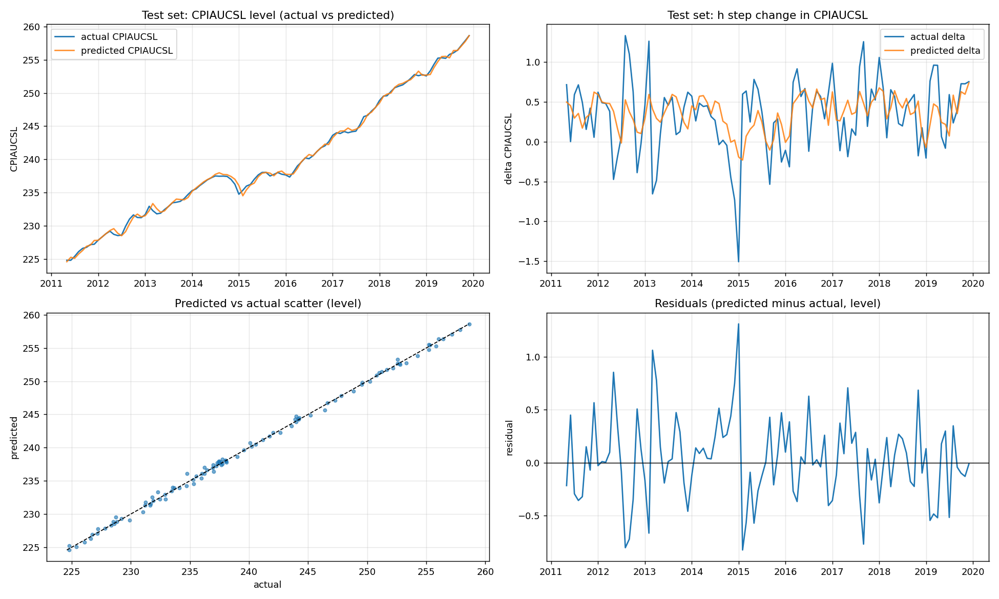 Test set predictions and residuals. The level plot in the top left looks great. The delta plot in the top right is the one to actually look at.
The level plot flatters the model. The two lines hug each other because most of \(\text{level}[t+h]\) is just \(\text{level}[t]\), which the model is handed for free: it only has to predict the change and add it to this month’s known CPI value.
The plot that actually tells you something is the delta plot, the predicted h step change against the actual h step change. This is where the model has to earn its keep, and the delta MAPE is 140% because actual deltas are often very close to zero and ratios blow up. The delta RMSE is 0.39, which is the same number as the level RMSE, and that is the point. The level RMSE is just the delta error sitting on top of a perfectly known value. Decompose like this:
\[\widehat{\text{CPI}}_{t+h} - \text{CPI}_{t+h} = (\text{CPI}_t + \widehat{\Delta y}) - (\text{CPI}_t + \Delta y) = \widehat{\Delta y} - \Delta y\]The level error is identically the delta error. Reporting the level metric without the delta metric is basically a magic trick.
This is also where the black box question comes in. An LSTM with 60,000 parameters is not interpretable in the way a regression coefficient is interpretable. You cannot point at a number and say “a one standard deviation increase in industrial production raises forecasted inflation by such and so.” You can run permutation importance on the inputs after training, you can compute integrated gradients along the input sequence, you can run partial dependence on a single feature while holding the others at their median. All of those are post hoc and approximate.
The natural next question is whether this approach extends to longer horizons, and whether you can get cleaner generalization by changing the inductive bias.
There are also obvious modifications to the architecture: attention over the input window, a state space layer in place of the LSTM, a probabilistic head that returns a distribution rather than a point estimate. Each of these changes the bias variance tradeoff in a different direction.
So where does this leave the original question? Honestly, this version doesn’t answer it yet. The level metrics look great for reasons that have nothing to do with the LSTM, the validation loss is worse than predicting the mean, and I haven’t put a simple autoregression on the same test set to compare against. That comparison is the next thing to do: fit an AR(p) and a random walk (predict a change of zero) on the differenced CPI series and report their delta RMSE next to the LSTM’s. Until the LSTM beats those, the honest conclusion is that monthly macro data is noisy enough that the extra machinery isn’t paying for itself. I still think there’s room for neural networks here, probably alongside econometric methods rather than instead of them, but this post is a starting point and not proof.