Eight Puzzle: State Space Search and the Cost of Heuristic Choices
Everyone’s familiar with the classic 8 Puzzle game:
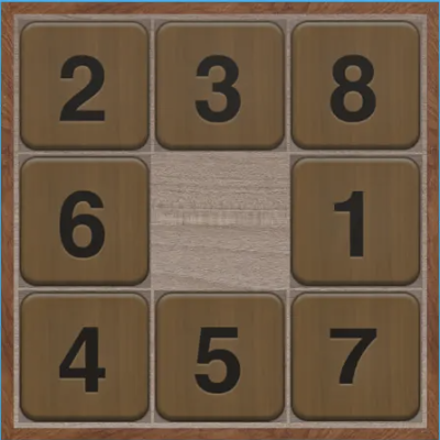
Slide tiles into the blank space until the numbers run 1 through 8 in order, with the blank in the top left.
Does the textbook hierarchy of state space search algorithms actually behave the way the textbooks claim on a problem small enough to inspect by hand? That’s what I wanted to find out here. The Eight Puzzle is the canonical toy. A 3x3 grid with eight numbered tiles and a single blank, and the goal is to slide tiles into ascending order with the blank in the top left. The reachable state space has size 181,440, which is exactly half of 9! because tile slides preserve permutation parity.
\[|S| = \frac{9!}{2} = 181{,}440\]So do random, breadth first, depth first, greedy best first, and A* search separate cleanly on this problem, and how much of the separation comes from the algorithm versus the heuristic you give it?
The problem is that the state space, while finite, is large enough that uninformed search wastes most of its work on configurations no human solver would ever consider. A blind frontier expansion at depth 18 still has roughly \(3^{18}\) candidates if you ignore cycle detection, which is around 387 million.
\[N(d) \leq b^d, \qquad b = 3, \, d = 18 \;\Longrightarrow\; N \approx 3.87 \times 10^8\]Even after pruning cycles the count stays in the millions on the harder boards. Any algorithm that does not somehow weight the search toward goal-like states is going to spend almost all of its budget visiting irrelevant ones. That is the case for heuristic search. The flip side is that a poorly chosen heuristic can make things worse than no heuristic at all, by confidently steering the search down a corridor that does not lead to the goal.
It’s a bit hard to explain the exact code implementation, so contact me if you want a more detailed explanation and I’d be happy to talk about it. The gist is this:
The dataset is three text files of starting configurations, grouped by the optimal solution length: 5_moves.txt, 18_moves.txt, and 27_moves.txt. Each file has ten boards encoded as a permutation of the digits 0 through 8, where 0 is the blank. The optimal length is the labeled difficulty. The 5 move set is for sanity checks. The 18 move set is the regime where uninformed search is on the edge of feasible. The 27 move set is past it.
The first thing you have to decide is how to represent a board. I went with
a 2D list of integers and tracked the blank position explicitly as
(blank_r, blank_c) so I never have to scan for it.
The constructor takes a 9 character digit string and fills the grid row by row.
\[\mathbf{B}(r, c) = \text{int}\!\left(\text{digitstr}[\,3r + c\,]\right)\]Tracking the blank position is not strictly necessary but it converts every move from \(O(n)\) to \(O(1)\), and over millions of generated successors that is a huge benefit.
A move slides the blank in one of four directions. Internally I shift the blank coordinate, check it stays inside the grid, and if so swap the blank with the tile that was there:
\[\begin{aligned} (r', c') &= (r, c) + d \\ \text{tiles}[r][c], \, \text{tiles}[r'][c'] &= \text{tiles}[r'][c'], \, \text{tiles}[r][c] \end{aligned}\]where \(d \in {(-1, 0), (1, 0), (0, -1), (0, 1)}\) for up, down, left, right. If the new coordinates are off the grid, the move is rejected.
\[\text{valid}(r', c') \iff 0 \leq r' \leq 2 \;\wedge\; 0 \leq c' \leq 2\]A State wraps a Board with three extra fields: a predecessor pointer, the move that produced this state, and the depth in the search tree.
\[s = (\mathbf{B}, \, \text{pred}, \, m, \, g), \qquad g(s) = \begin{cases} 0 & \text{pred} = \varnothing \\ g(\text{pred}) + 1 & \text{otherwise} \end{cases}\]The predecessor pointer is what lets me reconstruct the move sequence at the end without storing the full path inside the state. It also lets me detect cycles incredibly easily by walking back up the chain and checking for board equality.
\[\text{cycle}(s) \iff \exists \, s' \in \text{ancestors}(s) : \, s'.\mathbf{B} = s.\mathbf{B}\]This matters because without cycle detection, even BFS will waste time re-expanding the same configurations.
Successor generation tries all four directions on a copy of the board, keeps the moves that succeed, and wraps each into a new State with the predecessor set to self.
\[\text{succ}(s) = \left\{\, (\text{apply}(s, m), \, s, \, m, \, g(s) + 1) \,:\, m \in M, \; \text{valid}(s, m) \,\right\}\]The branching factor is at most four, typically two or three after cycle pruning.
\[2 \leq \big|\,\text{succ}(s) \setminus \{s' : \text{cycle}(s')\}\,\big| \leq 4\]The search abstraction is a Searcher base class with a list of untested states, a depth limit, and a tested counter. The contract is that find_solution pops a state via next_state, checks goal, generates successors otherwise, and adds them subject to a should_add filter that enforces the depth limit and rejects cycle creators.
\[\text{should\_add}(s) \iff \big(\, g(s) \leq L \;\vee\; L = -1 \,\big) \,\wedge\, \neg\,\text{cycle}(s)\]Subclasses override next_state to implement different orderings: random pick for the base class, FIFO for BFS, LIFO for DFS, and a priority-max pick for the informed searchers.
\[\text{next\_state} \in \begin{cases} \text{Uniform}(F) & \text{Random} \\ \arg\min_{s \in F} \, t_{\text{enq}}(s) & \text{BFS} \\ \arg\max_{s \in F} \, t_{\text{enq}}(s) & \text{DFS} \\ \arg\max_{s \in F} \, \text{priority}(s) & \text{Greedy, A*} \end{cases}\]There is a real argument for just running BFS and calling it done, because BFS is complete and optimal for unit-cost step problems, and the Eight Puzzle is one.
\[T_{\text{BFS}} = O(b^d), \qquad \text{return } s^* \;\text{with}\; g(s^*) = \min_{s \in \text{Goals}} g(s)\]The question is whether you can do better in states tested without giving up optimality. That is what informed search is supposed to deliver. An admissible heuristic should let A* prune the frontier without ever closing off the optimal path.
\[h \text{ admissible} \iff \forall \, s \in S: \; h(s) \leq h^*(s)\]The heuristics I implemented are non standard and worth describing. h0 returns 0, which makes A* behave like uniform cost search. h1
returns state.num_moves, which is the g cost and not a heuristic in the
usual sense. h2 returns num_moves plus the Manhattan distance of the
blank from the origin (0, 0).
Neither h1 nor h2 estimates the distance from the current state to the goal in the way a textbook heuristic would. I left them in because the experiments they enable still illustrate the point: any monotone signal that grows with depth or distance from a fixed reference biases the search, and the bias either helps or hurts depending on whether the signal correlates with proximity to the goal.
One thing to be upfront about: h1 and h2 are not admissible. Both include g, the number of moves already made, and that can easily be larger than the number of moves left to the goal. So the textbook optimality guarantee for A* does not formally apply to them. As you’ll see below, A* with h2 still returns optimal solutions here, but for a different reason.
The Greedy searcher computes priority as
\[\text{priority}(s) = -\left( \, \text{misplaced}(s) + h(s) \, \right)\]with h treated as zero unless the heuristic is h2, in which case it is added.
\[\text{misplaced}(s) = \begin{cases} 0 & \mathbf{B} = \mathbf{G} \\ \displaystyle\left(\sum_{r=0}^{2}\sum_{c=0}^{2} \mathbf{1}\!\left[\mathbf{B}(r,c) \neq \mathbf{G}(r,c)\right]\right) - 1 & \text{otherwise} \end{cases}\]The negation is there because I take max over priorities to pick the next state. Misplaced tile count, defined as the number of tiles not in their goal position, ends up doing basically everything Greedy. It is a real heuristic in the textbook sense, and Greedy with misplaced tile count finds solutions quickly but rarely optimally.
The A* searcher computes priority as
\[\text{priority}(s) = -\left( \, h(s) + \text{num\_moves}(s) \, \right)\]which is the negated f-cost from the textbook formula \(f = g + h\), if you read num_moves as g and h as the heuristic.
\[f(s) = g(s) + h(s), \qquad g(s) = \text{num\_moves}(s)\]The catch is that with h1 the h term is itself num_moves, so f effectively doubles g and the search degenerates into BFS with a strange tiebreaker.
\[f_{h_1}(s) = g(s) + h_1(s) = 2 \, g(s)\]With h2 things improve, because the blank distance term breaks ties in a way that prefers states whose blank is closer to the top left corner, which is where the goal puts it. On these particular puzzles that correlates with progress.
\[f_{h_2}(s) = 2 \, g(s) + |\text{blank}_r(s)| + |\text{blank}_c(s)|\]Notice that 2g goes up by 2 with every move, while the blank term only ranges from 0 to 4. So A* with h2 still mostly expands states in order of depth, like BFS, with the blank position deciding the order within and between neighboring depths. That is why it keeps finding optimal solutions even though h2 isn’t admissible.
Now to the results:
On 5_moves.txt every algorithm solves every puzzle. The interesting numbers are states tested. BFS expands on the order of a hundred to a few hundred states per puzzle. DFS with no depth limit can dive deep and tested counts are either small or huge depending on the seed. Greedy with misplaced tiles finishes in tens of states. A* with h2 finishes in similar territory. At this difficulty the algorithms are indistinguishable from a solving perspective.
On 18_moves.txt the separation between algorithms appears. BFS finishes but the expanded frontier crosses 100,000 states on the harder boards. DFS with a depth limit of 20 sometimes returns a 20 move solution and sometimes runs out of frontier without finding one. Greedy with the misplaced tile count finds solutions quickly but they are bad: 92, 56, 66, 186, 194, 96 moves on the puzzles it solves, against an optimal of 18.
\[\bar{g}_{\text{Greedy}} = \frac{92 + 56 + 66 + 186 + 194 + 96}{6} = 115, \qquad g^* = 18, \qquad \frac{\bar{g}}{g^*} \approx 6.4\]That is what greedy looks like. It commits to the first frontier expansion that scores well and then meanders.
A* with h2 gives the best results of the bunch. On the six boards it solves within a reasonable interrupt threshold, every solution is exactly 18 moves, and the states tested counts are 34413, 32283, 46097, 32009, 39396, 33053.
\[\bar{N}_{\text{tested}}^{A^*, h_2} = \frac{34413 + 32283 + 46097 + 32009 + 39396 + 33053}{6} \approx 36{,}209\]Compare to the BFS frontier on the same problem and A* tests fewer states on average. More importantly, every solution it returns is optimal, which Greedy never guarantees.
\[\forall \, i \in \text{solved}: \; g_{A^*, h_2}(s_i^*) = g^*(s_i)\]The four boards it does not solve are ones where I ran out of patience and interrupted the search rather than ones where the algorithm failed in principle.
 Algorithm comparison across difficulty levels. BFS and A track each other on optimality. Greedy diverges as soon as the optimal length crosses the easy threshold.*
The 27_moves.txt file is past the point where any of these algorithms reach a solution in a reasonable wall clock time without a much stronger heuristic. A heuristic that does not estimate distance to goal cannot, in general, prune deep enough to reach a 27 move target. If I wanted to push the difficulty further I would replace h2 with the sum of Manhattan distances of every tile from its goal position, which is admissible and well known to be effective on this problem.
\[h_{\text{MD}}(s) = \sum_{i=1}^{8} \big| r_i(s) - r_i^* \big| + \big| c_i(s) - c_i^* \big|\]It is worth asking whether the algorithm comparison generalizes. The answer is mostly yes. BFS is optimal but computationally expensive. DFS is computationally cheap but unreliable without an extremely good depth limit. Greedy is fast but lossy on solution quality. A* with an admissible heuristic is the one that guarantees optimality while searching less than BFS, and it pays for that with sensitivity to the heuristic.
\[h \leq h^* \;\Longrightarrow\; \text{A*\;optimal}\]The “searching less” part needs a caveat. If the heuristic is also consistent (it never drops by more than 1 across a single move), A* never expands more states than uniform cost search, ties aside. That isn’t a guarantee for every heuristic, and it’s not what my h2 runs show, since h2 is neither admissible nor consistent. The smaller counts I got come from the tiebreaking described above.
The 8-puzzle is small enough that you can see all four behaviors on a single laptop in a few minutes of runtime.
The A* with h2 numbers on 18_moves.txt make informed search look like an obvious win, but they don’t tell the whole story. On the boards it failed to solve in the same file, the blank’s position happens to be a poor proxy for true distance to the goal. On those, the priority queue keeps preferring states that score well by the heuristic but are actually further from the goal in moves.
\[h(s) \text{ small} \;\not\!\Longrightarrow\; h^*(s) \text{ small}\]Replacing the heuristic with sum of Manhattan distances might close the gap. It might be something I look into as an extension to this in the future.
The natural extensions from here are obvious. Implement the standard admissible heuristics inside A* (misplaced tiles without the g term, total Manhattan distance, linear conflict). Add iterative deepening A*, which trades memory for some redundant work and can solve 27 move boards on a laptop. Move from the 8-puzzle to the 15-puzzle, where the state space jumps from 181K to roughly \(10^{13}\) and uninformed search is no longer an option at all.
\[|S_{15}| = \frac{16!}{2} \approx 1.05 \times 10^{13}\]The result of this exercise is that the algorithm hierarchy mostly behaves as expected, and that the heuristic matters as much as the algorithm. Even a weak heuristic like h2 was enough to beat BFS in the 18 move regime, but not enough to push to 27. That needs a heuristic that actually estimates distance to the goal.